Motivation

The product of two (d)-degree polynomials is a polynomial of degree (2d), i.e. if (A(x)=a_0+a_1x+a_2x^2+\ldots+a_dx^d) and (B(x)=b_0+b_1+b_2x^2+\ldots+b_dx^d) then

\[A(x)B(x)=a_0b_k+a_1b_{k-1}+\ldots+a_kb_0=\sum_{i=0}^{k}a_i b_{k-i}\]

Computing (c_k) from this formula takes (O(k)) steps aand finding all (2d+1) coefficients would therefore take (\Theta(d^2))

A degree-(d) polynomial is uniquely characterized by its values at any (d+1) distinct points.

We can represent a degree-(d) polynomial (A(x)) by either (i) it’s coefficients (a_0, a_1,\ldots a_d) or (ii) the values (A(x_0), A(x_1),\ldots A(x_d))

In the second representation polynomial multiplication takes linear time.

Evaluation by divide-and-conquer

If we choose the (n) points for evaluation of (A(x)) as:

\[\pm x_0, \pm x_1, \ldots, \pm x_{n/2-1}\]

then the computatin required for each (A(x_i)) and (A(-x_i)) overlap a lot because the even powers of (x_i) coincide with those of (-x_i).

\[A(x)=(a_0+a_2x^2+a_4x^4+\ldots)+x(a_1+a_3x^2+\ldots) A(x)=A_{\rm even}(x^2)+xA_{\rm odd}(x^2)\]

hence

\[A(x_i)=A_e(x_i^2)+x_iA_o(x_i^2) A(-x_i)=A_e(x_i^2)-x_iA_o(x_i^2)\]

Noew we need to evaluate (A_e(x)) and (A_o(x)) (which each have half the degree of (A(x))) at just (n/2) points, (x_0^2,\ldots x_{n/2-1}^2).

If we could recurse then time complexity would be (T(n)=2T(n/2)+O(n)\implies O(n\log n)). The plus-minus trick only works at the top level of the recursion. To recurse at the next level, we need the (n/2) evaluation points (x_0^2, x_1^2,\ldots x_{n/2-1}^2) to be themselves plus-minus pairs. For this we take (n^{\rm th}) roots of unity as the evaluation points.

Interpolation

We have (\rm \langle values\rangle = FFT(\langle coefficients\rangle, \omega)). where the complex roots of unity are ({1,\omega,\omega^2,\ldots,\omega^{n-1}})

We have:

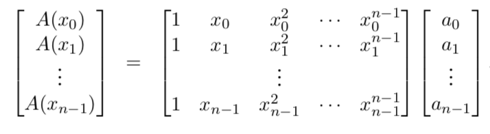
Call the matrix in the middle (M). Its specialized format - a Vandermonde matrix gives its many remarkable properties

If (x_0, \ldots x_{n-1}) are distinct numbers, then (M) is invertible. Vandermonde matrices are quicker to invert than more general matrices in (O(n^2)) instead of (O(n^3)). However, this is still not fast enough so we turn to complex roots of unity.

Interpolation resolved

The FFT multiplies an arbitary (n)-dimensional vector (coefficient representation) by the (n\times n) matrix

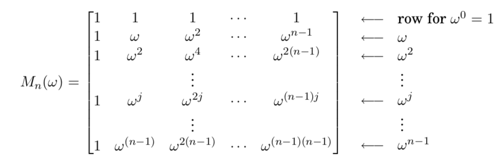
It’s ((j,k)^{\rm th}) entry is (\omega^{jk}). The columns of (M) are orthogonal to each other and are called Fourier basis.

Take (\omega=e^{2\pi i/n}) and (\langle u, v\rangle = u_0\overline{v_0}+u_1\overline{v_1}+\ldots u_{n-1}\overline{v_{n-1}}) where (\overline {re^{i\theta}}=re^{-i\theta}).

Multiplication of columns (j) and (k) of matrix (M) gives

\[1+\omega^{j-k}+\omega^{2(j-k)}+\ldots+\omega^{(n-1)(j-k)}=\frac{(1-\omega^{n(j-k)})}{(1-\omega^{j-k})}\]

which is a Geometric series which is (0) except (j=k) in which case all terms are (1) and sum is (n).

Thus (M\overline {M}=nI) or (M^{-1}=\frac 1n\overline {M}). The ((j, k)^{\rm th}) entry of (\overline M) is the complex conjugate of the correspoding entry of (M), i.e. (\omega ^{-jk}). So (\overline {M}=M_n(\omega^{-1}))

So we have ( \langle {\rm coefficient}\rangle = \frac 1n \rm FFT(\langle values\rangle, \omega^{-1}))