Self-adjusting binary trees that work in (O(\log n)) amortized time bound. The operation performed is the splay operation.

For a splay operation at node x: ((p(x)) is the parent of (x))

Case (a): If (x) has a parent but no grandparent we rotate at (p(x)).
Case (b): If (x) has a grandparent and both (x) and (p(x)) are both left or right childrenn, we rotate at (p^2(x)) and then at (p(x)).
Case (c): If (x) has a grandparent and (x) is a left and (p(x)) is a right child, or vice versa, we rotate at (p(x)) and then at the new parent of (x).

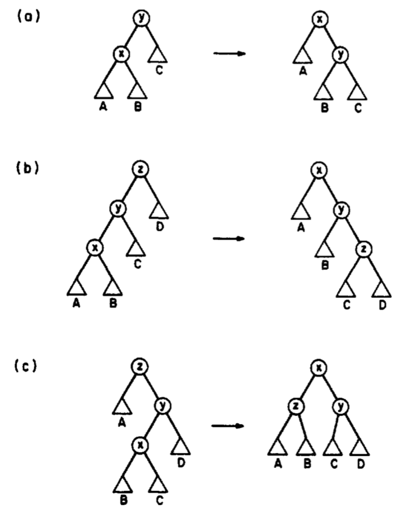
This moves (x) to the root of the tree while rearranging the rest of the original path to (x).

We perform a splay operation during each access or update operation. Using amortized time analysis for (m) operations total time taken is (O(m\log n)) or (O(\log n)) amortized time per operation.

Amortized Time Analysis

Let (T) be a tree of (n) nodes. For node (v\in T) let (n_T(v)) ve the number of nodes in the subtree of (v) including (v).

We define the potential function (\phi(T)=\sum_{v\in T}r_T(v)) where (r_{T}(v)=\log {2}\lfloor n{T}(v)\rfloor).

For a completely skewed tree it will be (\log_2n+\log_2(n-1)+\ldots \log_21=O(n\log n)).

For a completely balanced tree of height (h) it will be (\sum_{i=0}^h2^i\log_2(2^{h-i+1})=\sum_{i=0}^h2^i(h-i+1)=O(n))

Suppose the tree undergoes (m) searches for keys (k_{i_1},k_{i_2},\ldots k_{i_m}) starting from tree (T_0) and after searching for (k_{i_1}) to (T_1) and so on until (T_m).

Let actual cost of (i^{\rm th}) search be (c_i) and amortized cost of (i^{\rm th}) search be (\hat c_i=c_i+\phi(T_i)-\phi(T_{i-1})). We claim that (\hat{c}_{i} \leqslant 3 \log _{2} n). Hence actual cost becomes \(\begin{align} \sum_{i=1}^mc_i&=\sum_{i=1}^m[\hat c_i+\phi(T_{i-1})-\phi(T_i)]\\ &=\sum_{i=1}^m\hat c_i+\sum_{i=1}^m(\phi(T_{i-1}-\phi(T_i)))\\ &=\sum_{i=1}^m\hat c_i+[\phi(T_0)-\phi(T_m)]\\ &=\sum_{i=1}^m\hat c_i+n\log n\\ &\le3m\log n+n\log n\\ &\le 4m\log n\tag{\(m\ge n\)} \end{align}\)

Now we prove (\hat{c}_{i} \leqslant 3 \log _{2} n) for various cases. (r’) represents the rank after rotation.

Lemma If (a+b\le c) then (\log a+\log b\le 2\log c-2) since (ab\le c^2/4) where (c^2\ge (a+b)^2\ge 4ab) using AM-GM inequality.

Case (a) (zig)

Total cost involves 1 rotation and potential change. We have (r’(x)=r(y)) so (\Delta \phi=(r’(x)+r’(y))-(r(x)+r(y))=r’(y)-r(x)\le r’(x)-r(x)) as (y) has less nodes afterwards and less rank. So (\hat c_i\le 1+(r’(x)-r(x))\le 1+3(r’(x)-r(x)))

Case (c) (zig-zag)

Total cost involves 2 rotation and potential change (\Delta \phi=r’(x)+r’(y)+r’(z)-r(x)-r(y)-r(z))

Here (\hat c_i=2+(r’(x)-r(x))+r’(y)+r’(z)-r(y)-r(z))

Also (n’(y)+n’(z)= n’(x)-1\le n’(x)). Using the lemma (\log (n’(y)) + \log (n’(z))\le 2\log (n’(x))-2) or (r’(y)+r’(z)\le 2r’(x)-2).

So we have (\hat c_i\le 2+ (r’(x)-r(x))+(2r’(x)-2)-r(y)-r(z)) or (\hat c_i\le (3r’(x)-r(x)-r(y)-r(z)). Also we have (r(z)=r(x)) and (r(y)\ge r(x)) so (\hat c_i\le 3(r’(x)-r(x)))

Case (b) (zig-zig)

Total cost involves 2 rotation and potential change

Similar to case (c) we have (\hat c_i=2+(r’(x)-r(x))+r’(y)+r’(z)-r(y)-r(z)) and (n(x)+n’(z)+1=n’(x)) giving (r(x)+r’(z)\le 2r’(x)-2) or (r’(z)\le 2r’(x)-r(x)-2)

So we have (\hat c_i\le 2+(r’(x)-r(x))+r’(y)+(2r’(x)-r(x)-2)-r(y)-r(z)) or (\hat c_i\le (3r’(x)-2r(x))+r’(y)-r(y)-r(z)). Also we have (r(z)=r’(x)) and (r(y)\ge r(x) ) giving (\hat c_i\le 3(r’(x)-r(x))-\underbrace{(r(z)-r’(y))}_{>0}\ge 3(r’(x)-r(x)))

Conclusion

If we have (d) splays then (\hat c=\sum_{i=1}^d\hat c_i\le \sum_{i=1}^d3(r_i(x)-r_{i-1}(x))=3(r_d(x)-r_0(x)))

The maximum change in rank can be (\log n) giving (\hat c\le 3\log n)